Taxi fare problem? What is this about?
If you have attended any Oracle-related conference lately, you've probably noticed a surge in machine learning (ML) related talks. This, of course, comes along with several big data (BD) related ones and, finally, Oracle RDBMS-based artificial intelligence (AI) embedded features, which led to this experiment of mine. Yes, well, but what is this "Taxi Fare" problem? If you are reading this you are probably an Oracle DBA or something like that and, admit it, us Oracle guys are quite Oracle-focused, even though we usually look around to see what others are doing. I have looked in Google's direction, more specifically in the BD and ML fields. Thanks to Pythian's internal training program, I was able to take a course about these subjects and there I encountered the Taxi Fare prediction problem. This problem has been described in many places much better than I am able to, so I'll present a summary: if provided with the start and end points of taxi rides in New York, the date of the ride and the final amount paid, plus several other pieces of data, can we predict the taxi fare for a proposed ride? In more formal terms: this is a typical prediction model usually resolved with a regression model approach. Sounds easy, but it is not.The data
As almost everybody in the BD and AI business knows, one of the most important steps in getting value from the data is to prepare it for analysis. This is particularly important for ML algorithms because we are training our model and we want the data to show an accurate picture of what we have or else it will produce wrong results. I've obtained a publicly available data set in CSV format and imported it into my laboratory database in two sets: one of two million rows and another with the whole 54 million rows. The train data table includes the following columns:Name Null? Type
----------------- ----- -------------
FARE_AMOUNT NUMBER(8,4)
PICKUP_DATETIME TIMESTAMP(6)
PICKUP_LONGITUDE NUMBER(25,22)
PICKUP_LATITUDE NUMBER(25,22)
DROPOFF_LONGITUDE NUMBER(25,22)
DROPOFF_LATITUDE NUMBER(25,22)
PASSENGER_COUNT NUMBER(38)
Data preparation
As I mentioned above, most AI experts say that preparing the data for our model is the key to obtaining the best results. Why? Because the data reflects the world as the model sees it. In our case, if we are analyzing taxi trips in New York City, why would the data include coordinates for Madrid? Or coordinates that make no sense such as longitude values outside of the -180º/180º range? What comes in handy here is the Oracle Data Miner SQL*Developer extension, or more precisely, the "Explore Data" component. This component analyzes the data and provides some basic statistics about each of the columns such as min, max, average or median. This is very useful to spot data issues such as negative fare amounts or coordinates that do not fall in the New York City area. There are also tools to chart the data, extract features and, of course, to create models, among others. [caption id="attachment_105679" align="aligncenter" width="150"]
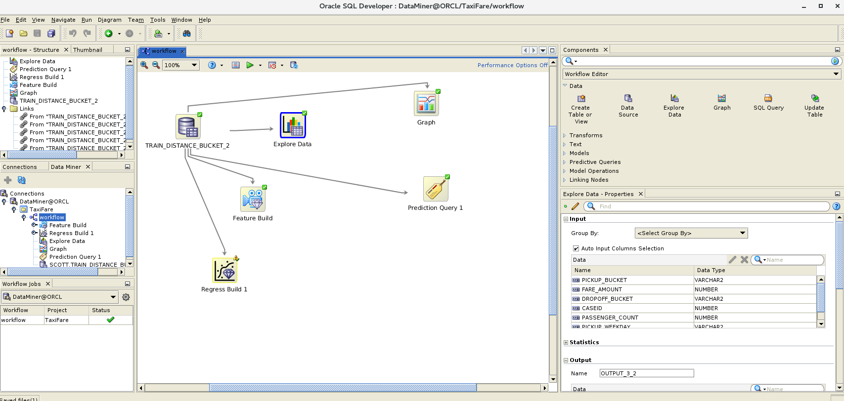
SQLDeveloper Data Miner[/caption] The person or team who knows what the data brings is also very important because they add the most value. While the taxi fare problem is very generic, for more specific business data such as pharmaceutical molecules or tuna migration routes, having someone who really knows the business and understands the data is critical. It is critical for the DBA (or data scientist) to work with this person or team in order to obtain the maximum value out of the model and tune it accordingly.
What to look for?
Back to our taxi rides; we have dates, coordinates, fares and the number of passengers per ride. There are a couple of easy ones here, right? New York City coordinates are 40ºN 74ºW, so in order to keep things simple, I've assigned a range of 35º to 45º for latitude and -80º to -70º for longitude as valid data ranges. Every row that refers to coordinates outside of these boundaries has been deleted. The other easy one is the fare amount. Negative fare? No way and, now that I think of it, a negative number of passengers? Not a good idea either, so all these rows have been deleted as well. It is interesting to mention that a person who knows the business may not think of these cases simply because they make no sense, but for those of us who "Love your data"™, it is obvious that data can have errors, either human or machine induced, and it is our job to take care of them. Finally, the pickup date and time is an interesting piece of data. In order to improve the model, we can make sure that we know exactly what time range we are talking here so we don't hit any statistical oddities, such as a very long taxi drivers strike or a natural phenomenon that may have altered the behavior of the NYC citizens for a couple of months. And also, we don't want to take into account things like the taxi rides of the early 1930's, so we may want to make sure that we are working only with data that makes sense in time. Due to the process I used to load the public data into my sandbox Oracle database, all the dates that were not actual dates have been automatically removed, which is a necessary data cleansing task. I also made sure that the rides occurred in the last decade, so we should be fine here. So far, we've done only data cleansing; that is, making sure that the data we have makes sense for our particular business case and that it reflects the world as we want our model to see it. What comes next?Data transformations
While it is cool to have the tiniest details of a given taxi ride, this is the XXI century and we collect exabytes of data every second, it is not so useful to train a model. A simple example. We have the pickup time down to the minute but does it really matter if a taxi ride started at 2:00 PM or at 2:10 PM? The answer is "it depends." If we are looking for some very detailed analysis of the traffic flows to cross-reference with traffic jams, red lights and accidents, then yes, it is relevant. But for our current needs, no way. Even more, we can fall in the pit of overfitting our model. So in this particular case, I've opted for scaling up the pickup time to weekday and instead of using a date data type, I transformed this to a three-character string because ML algorithms seem to prefer data in strings, or categorized, rather than in continuous values, or non-categorized. This is not my idea but rather a standard way to transform date data for easy categorization by the model. Next is the coordinates data. Again, it does not matter much a few arch seconds up or down in the map, but the general geographical area within the city is still important. This is mainly because of routes with more bridges, which means tolls, routes that start or end at an airport, routes with fixed fares and that kind of stuff. Here again, avoiding the detailed coordinates information both reduces the chances of overfitting the model and improves the accuracy based on neighborhoods that may include special cases. There is, of course, a data transformation technique to deal with these cases. The idea, again, is to get rid of the details in the pickup and dropoff coordinates by grouping them into, in this case, artificially created city areas or squares. This creates a matrix and assigns a code to all the coordinate pairs that pertain to a given square, hence categorizing our pickup and dropoff points. Finally, I added a new column to the data, a new feature, to store the geographical distance between the pickup and dropoff points. This piece of information is important in our model because there are relatively short rides with quite high fares which goes against the principle of longer distance and time equal a higher fare. These cases appear due to the fixed fares to and from the airports, so the distance, even the simplest linear calculation used here, is a relevant feature for our model. This again is achieved with an Oracle option called Spatial and Graph. This option includes the SDO_GEOMETRY type which allows these kinds of calculations to be simple to code in SQL while remaining accurate. As a last step for the data preparation, I added a column called CASEID. This is not a feature for our model but a primary key added to the table to uniquely identify the cases in our data, following the recommendations in the Oracle Data Mining documentation. This is the query I used to transform the data. It takes care of adding the CASEID column, classifies the pickup date into a weekday, "bucketizes" the pickup and dropoff coordinates into zones and calculates the linear distance between pickup and dropoff points in kilometres (yes, I am European ;) ).INSERT /*+ APPEND PARALLEL(4) */ INTO TRAIN_DISTANCE_BUCKET
SELECT /*+ PARALLEL(4) */
ROWNUM AS CASEID,
T.FARE_AMOUNT,
TO_CHAR(T.PICKUP_DATETIME,'DY') PICKUP_WEEKDAY,
'Z'||CASE
WHEN
(PICKUP_LONGITUDE BETWEEN -76 AND -75
AND
PICKUP_LATITUDE BETWEEN 40 AND 41) THEN 1
WHEN
(PICKUP_LONGITUDE BETWEEN -75 AND -74
AND
PICKUP_LATITUDE BETWEEN 40 AND 41) THEN 2
WHEN
(PICKUP_LONGITUDE BETWEEN -74 AND -73
AND
PICKUP_LATITUDE BETWEEN 40 AND 41) THEN 3
WHEN
(PICKUP_LONGITUDE BETWEEN -73 AND -72
AND
PICKUP_LATITUDE BETWEEN 40 AND 41) THEN 4
WHEN
(PICKUP_LONGITUDE BETWEEN -76 AND -75
AND
PICKUP_LATITUDE BETWEEN 39 AND 40) THEN 5
WHEN
(PICKUP_LONGITUDE BETWEEN -75 AND -74
AND
PICKUP_LATITUDE BETWEEN 39 AND 40) THEN 6
WHEN
(PICKUP_LONGITUDE BETWEEN -74 AND -73
AND
PICKUP_LATITUDE BETWEEN 39 AND 40) THEN 7
WHEN
(PICKUP_LONGITUDE BETWEEN -73 AND -72
AND
PICKUP_LATITUDE BETWEEN 39 AND 40) THEN 8
WHEN
(PICKUP_LONGITUDE BETWEEN -76 AND -75
AND
PICKUP_LATITUDE BETWEEN 38 AND 39) THEN 9
WHEN
(PICKUP_LONGITUDE BETWEEN -75 AND -74
AND
PICKUP_LATITUDE BETWEEN 38 AND 39) THEN 10
WHEN
(PICKUP_LONGITUDE BETWEEN -74 AND -73
AND
PICKUP_LATITUDE BETWEEN 38 AND 39) THEN 11
WHEN
(PICKUP_LONGITUDE BETWEEN -73 AND -72
AND
PICKUP_LATITUDE BETWEEN 38 AND 39) THEN 12
WHEN
(PICKUP_LONGITUDE BETWEEN -76 AND -75
AND
PICKUP_LATITUDE BETWEEN 37 AND 38) THEN 13
WHEN
(PICKUP_LONGITUDE BETWEEN -75 AND -74
AND
PICKUP_LATITUDE BETWEEN 37 AND 38) THEN 14
WHEN
(PICKUP_LONGITUDE BETWEEN -74 AND -73
AND
PICKUP_LATITUDE BETWEEN 37 AND 38) THEN 15
WHEN
(PICKUP_LONGITUDE BETWEEN -73 AND -72
AND
PICKUP_LATITUDE BETWEEN 37 AND 38) THEN 16
ELSE 0
END AS PICKUP_BUCKET,
'Z'||CASE
WHEN
(DROPOFF_LONGITUDE BETWEEN -76 AND -75
AND
DROPOFF_LATITUDE BETWEEN 40 AND 41) THEN 1
WHEN
(DROPOFF_LONGITUDE BETWEEN -75 AND -74
AND
DROPOFF_LATITUDE BETWEEN 40 AND 41) THEN 2
WHEN
(DROPOFF_LONGITUDE BETWEEN -74 AND -73
AND
DROPOFF_LATITUDE BETWEEN 40 AND 41) THEN 3
WHEN
(DROPOFF_LONGITUDE BETWEEN -73 AND -72
AND
DROPOFF_LATITUDE BETWEEN 40 AND 41) THEN 4
WHEN
(DROPOFF_LONGITUDE BETWEEN -76 AND -75
AND
DROPOFF_LATITUDE BETWEEN 39 AND 40) THEN 5
WHEN
(DROPOFF_LONGITUDE BETWEEN -75 AND -74
AND
DROPOFF_LATITUDE BETWEEN 39 AND 40) THEN 6
WHEN
(DROPOFF_LONGITUDE BETWEEN -74 AND -73
AND
DROPOFF_LATITUDE BETWEEN 39 AND 40) THEN 7
WHEN
(DROPOFF_LONGITUDE BETWEEN -73 AND -72
AND
DROPOFF_LATITUDE BETWEEN 39 AND 40) THEN 8
WHEN
(DROPOFF_LONGITUDE BETWEEN -76 AND -75
AND
DROPOFF_LATITUDE BETWEEN 38 AND 39) THEN 9
WHEN
(DROPOFF_LONGITUDE BETWEEN -75 AND -74
AND
DROPOFF_LATITUDE BETWEEN 38 AND 39) THEN 10
WHEN
(DROPOFF_LONGITUDE BETWEEN -74 AND -73
AND
DROPOFF_LATITUDE BETWEEN 38 AND 39) THEN 11
WHEN
(DROPOFF_LONGITUDE BETWEEN -73 AND -72
AND
DROPOFF_LATITUDE BETWEEN 38 AND 39) THEN 12
WHEN
(DROPOFF_LONGITUDE BETWEEN -76 AND -75
AND
DROPOFF_LATITUDE BETWEEN 37 AND 38) THEN 13
WHEN
(DROPOFF_LONGITUDE BETWEEN -75 AND -74
AND
DROPOFF_LATITUDE BETWEEN 37 AND 38) THEN 14
WHEN
(DROPOFF_LONGITUDE BETWEEN -74 AND -73
AND
DROPOFF_LATITUDE BETWEEN 37 AND 38) THEN 15
WHEN
(DROPOFF_LONGITUDE BETWEEN -73 AND -72
AND
DROPOFF_LATITUDE BETWEEN 37 AND 38) THEN 16
ELSE 0
END AS DROPOFF_BUCKET,
T.PASSENGER_COUNT,
SDO_GEOM.SDO_DISTANCE
(
SDO_GEOMETRY
(
-- THIS IDENTIFIES THE OBJECT AS A TWO-DIMENSIONAL POINT.
2001,
-- THIS IDENTIFIES THE OBJECT AS USING THE GCS_WGS_1984 GEOGRAPHIC COORDINATE SYSTEM.
4326,
NULL,
SDO_ELEM_INFO_ARRAY(1, 1, 1),
-- THIS IS THE LONGITUDE AND LATITUDE OF POINT 1.
SDO_ORDINATE_ARRAY(PICKUP_LONGITUDE, PICKUP_LATITUDE)
),
SDO_GEOMETRY
(
-- THIS IDENTIFIES THE OBJECT AS A TWO-DIMENSIONAL POINT.
2001,
-- THIS IDENTIFIES THE OBJECT AS USING THE GCS_WGS_1984 GEOGRAPHIC COORDINATE SYSTEM.
4326,
NULL,
SDO_ELEM_INFO_ARRAY(1, 1, 1),
-- THIS IS THE LONGITUDE AND LATITUDE OF POINT 2.
SDO_ORDINATE_ARRAY(DROPOFF_LONGITUDE, DROPOFF_LATITUDE)
),
1,
'UNIT=KM'
) DISTANCE_KM
FROM TRAIN T
So, after all these cleansing and transformations we have a table with the following columns:
Name Null? Type
 --------------- ----- ------------
 CASEID NUMBER
 FARE_AMOUNT NUMBER(8,4)
 PICKUP_WEEKDAY VARCHAR2(12)
 PICKUP_BUCKET VARCHAR2(41)
 DROPOFF_BUCKET VARCHAR2(41)
 PASSENGER_COUNT NUMBER(38)
 DISTANCE_KM NUMBER
And this is what the Data Miner Explore Data option shows: [caption id="attachment_105680" align="aligncenter" width="150"]
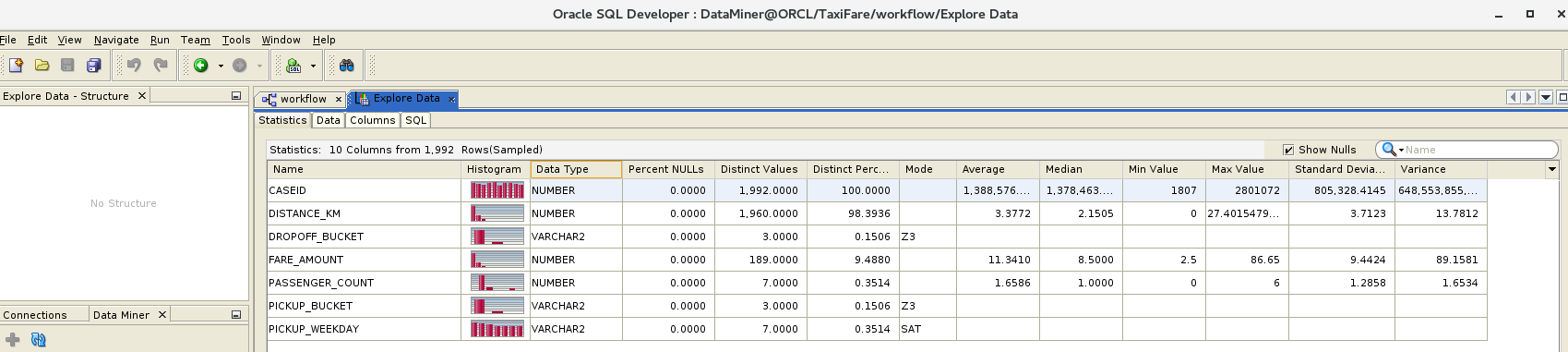
Data Miner Explore Data output[/caption]
And what do we have so far?
In the beginning, there was raw data in our database. For this experiment, I've loaded it from a public source but in a real-world scenario, it can be data that is already in your DWH or DSS or even your production OLTP database. Once the raw data was analyzed in statistical and more importantly, business logic terms, several cleansing and transforming actions were deemed necessary and executed on it. Out of these activities came the features we will be using in our model. After cleansing and transforming the data and storing it into a single table, we are ready to create our model.Model creation
Surprisingly enough, creating the model is pretty simple once one has decided what algorithm to use. The documentation is pretty straight forward in this regard. We start by selecting the Mining Function. Of all existing functions in 18c, I've chosen the regression function because it is the only predictive function available besides the time_series one. Then the algorithm. Again we have several choices available but only two match our needs: ALGO_GENERALIZED_LINEAR_MODEL and ALGO_SUPPORT_VECTOR_MACHINES. The former is a basic linear regression algorithm with the very important advantage that the calculations are relatively simple, although the results are not always as accurate. The latter, support vector machines, is the default regression algorithm used by Oracle in a ML model with its main advantage being that it is highly scaleable and usable, although it requires higher computational power than linear regression. Next comes data transformation. This is handy for live data where a transformation can be applied to the data on the model itself. This obviously means more processing time and resources are required but it may be useful if we can't have the data prepared earlier or if we opt for any of the automatic transformations Oracle features in the Data Mining component. In our particular case, we have already massaged the data for our purposes so we will ignore this optional setting. Once these two important configuration items have been established, we can proceed with the model settings. These are stored in a settings table and serve to tune the mining function and the data mining algorithm. There are global settings that modify the behaviour of the model. There are no specific settings for the regression data mining function but we have settings for the algorithm of our choice, in our case the generalized linear model. Finally, we have the Solver settings. Data Mining algorithms can use different solvers and their behavior can be tuned with these settings. Note how fast the model is created. After all, what we all want in a blog like this is some code, so here goes with some very simple DDL and a PL/SQL anonymous block that achieves the basic configuration of our model:CREATE TABLE linear_reg_taxi_fare_settings (
setting_name VARCHAR2(30),
setting_value VARCHAR2(4000));
BEGIN
INSERT INTO linear_reg_taxi_fare_settings (setting_name, setting_value) VALUES
(dbms_data_mining.algo_name, dbms_data_mining.algo_generalized_linear_model);
END;
/
------------------------ CREATE THE MODEL -------------------------------------
SQL> BEGIN
2 DBMS_DATA_MINING.CREATE_MODEL(
3 model_name => 'Lin_reg_taxi_fare',
4 mining_function => dbms_data_mining.regression,
5 data_table_name => 'TRAIN_DISTANCE_BUCKET',
6 case_id_column_name => 'caseID',
7 target_column_name => 'FARE_AMOUNT',
8 settings_table_name => 'linear_reg_taxi_fare_settings');
9 END;
10 /
PL/SQL procedure successfully completed.
Elapsed: 00:00:10.552
Note how fast the model creation was - only 10 seconds. This is partially due to the small number of rows I am using in this experiment, only 2 million, but also shows how fast the model creation/training is. Creating an identical model with 54 million rows took about 52 minutes. Still, not bad given that this is being executed on my i7, 16GB RAM, SSD laptop.
Working with Data Miner
When the data has been prepared to train our model, the Data Miner SQL Developer extension provides an interesting GUI to allow us to create a workflow graph to apply different transformations and data analysis models. It also provides tools to analyze the source data and, more importantly for this case, once the model has been created it provides performance information, not in terms of speed but in terms of accuracy or model fitness. With this in mind, I've created a couple workflows, one for the 2 million rows train data table and another for the 54 million rows one. The workflows are very simple and similar, aiming at creating only two regression models, i.e. linear generalized and support vector, and to obtain the data. An interesting option included is the possibility of scheduling the workflow node executions. This is interesting in a live production database where the data can change quite frequently in order to keep our data models up to date. As a simple example, I will delve deeper into the results in the second part of this series. Here is what a generalized linear vs. support vector machine model comparison looks like for the 2 million rows train data. [caption id="attachment_105778" align="aligncenter" width="150"]
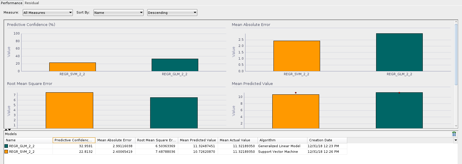
Generalized Linear versus Support Vector Machine performance comparison[/caption]
In the next episode...
- Put your new model to work. I have a model now, how do I use it?
- Review model performance metrics. Are my model predictions accurate?
- Pros and cons of this approach.
Continue reading with Episode 2.
Data Analytics Consulting Services
Ready to make smarter, data-driven decisions?
Share this
Share this